The renderers generate the images and spectral information from the 3D model and physical properties defined in the 3D Module and Physics Module.

In Shape there are several renderers that have quite different purposes and generate different types of output. Which one you will choose depends very strongly on the astrophysical problem that you aim to solve. The currently available renderers are the following:

Particle

Mesh

Transfer

Text

Grid

Purpose and short description (click on the renderers name to go to the more detailed description):

Particle: The Particle Renderer is for quick exploration of model structures and spectral models. It uses the particles assigned in the 3D Module to integrate their density values directly onto the image plane. If the emission from more than one particle falls into the same pixel, the emission from all of them is added together. No opacity is taken into account, i.e. objects are optically thin. This renderer is the fastest of all. The spatial resolution that can be achieved with this renderer depends on the number of particles used. For 64 bit systems with large amount of RAM, the number of particles can be more than a million, allowing rather high resolution.

Mesh: The Mesh Renderer directly uses the 3D mesh structure and transfers it to a regular 3D grid. The resulting images are smooth without the random particle noise characteristic of the Particle Renderer. Along with the spatial distribution of the mesh, the physical properties that depend on position in space are transfered to the grid. This is done for each mesh object from the 3D Module. Each object is then rendered separately onto the image. Similar to the Particle Renderer, no opacity is taken into account. The spatial resolution of this renderer depends on the the number of grid points used.

Transfer: The Transfer Renderer is used for physical radiation transfer calculations. It does not only perform a direct integration along the line of sight, but does also perform radiation transfer from any light sources in the object. It takes into account the physical properties of the objects as defined in Physics and 3D Modules. Its usage requires a good understanding of how which physical properties are available, as well as how they are defined and calculated in Shape. Similar to the Mesh Renderer it uses a regular grid and the 3D meshes to define the spatial structure of an object. For more details see the separate section on the Transfer renderer.

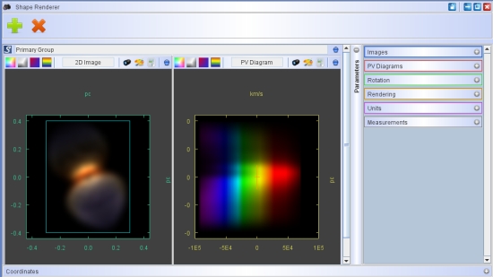
Text: The Text Renderer outputs an ASCII file with individual particle data as projected on the sky. These include brightness, but, most importantly, projected velocity vectors along and perpendicular to the line of sight. This allows to analyze with external programs not only the Doppler-shift, but also the transverse kinematics as a function of position. These data can also be plotted in various ways directly in the Plot Module.

Grid: The Grid Renderer uses the particles to sample the spatial properties of an object, but places them into a regular grid. If more than one particle ends up in a grid cell, then the properties are averaged. The Grid Renderer is also an optically thin renderer.

 

Common features:

Render modifiers or filters

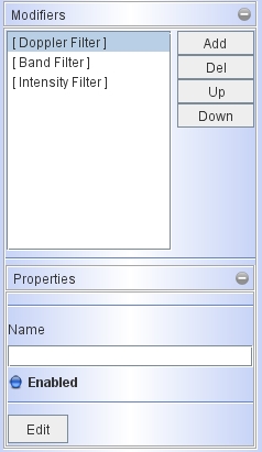
Shape allows you to perform several filter operations at render time. They select a certain range of values of a certain type for the output image. Currently there are three different filters available: Doppler, Band and Intensity. They are applied in a similar fashion as the modifiers in the 3D Module.You select and add them by clicking on the Add button. The order of the filters can changed by selected one and moving them Up or Down with the corresponding button. They can be delected using the Del button. Similar to the 3D modifiers, they can be Enabled and disabled without deleting.

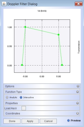
The filter characteristics can be set by clicking on the Edit button. It opens a graph dialog, where you can set the filter transmission as usual in the form of an analytic or manual function. For the manual graph you can load a set of values which represent measurements of your instrumental transmission. The Doppler filter is set in terms of velocity (km/s), the band filter in terms of wavelength (m) and the intensity filter is given in terms of power per solid angle (W/sr).

Example applications include taking into account limited filter ranges that exclude certain velocity ranges of a high speed explosion for given spectral lines (e.g. Ribeiro et al., 2009). The band filter can take into account complex spectral detector characteristics. The intensity filter lets you apply an arbitrary image look-up-table in terms of physical fluxes. The image modifiers are applied during rendering, before the image adjustment filters on the image view panels.